Performance
Maple 2019 improves the performance of many routines.
factor
Maple 2019 includes performance improvements for factoring sparse multivariate polynomials with integer coefficients.
> |
![vars := [seq(x[i], i = 1 .. 8)]](Performance/Performance_1.gif) |
> |
 |
> |
 |
> |
 |
The following factorization took about 5 seconds in Maple 2018 on the same machine.
> |
 |
memory used=40.03MiB, alloc change=41.09MiB, cpu time=250.00ms, real time=247.00ms, gc time=0ns |
![`*`(`+`(`*`(474, `*`(`^`(x[1], 5), `*`(`^`(x[3], 4), `*`(`^`(x[4], 3), `*`(x[5], `*`(`^`(x[6], 2))))))), `-`(`*`(429, `*`(`^`(x[1], 4), `*`(`^`(x[2], 2), `*`(x[3], `*`(`^`(x[6], 4), `*`(`^`(x[7], 3), ...](Performance/Performance_21.gif)
![`*`(`+`(`*`(474, `*`(`^`(x[1], 5), `*`(`^`(x[3], 4), `*`(`^`(x[4], 3), `*`(x[5], `*`(`^`(x[6], 2))))))), `-`(`*`(429, `*`(`^`(x[1], 4), `*`(`^`(x[2], 2), `*`(x[3], `*`(`^`(x[6], 4), `*`(`^`(x[7], 3), ...](Performance/Performance_22.gif)
![`*`(`+`(`*`(474, `*`(`^`(x[1], 5), `*`(`^`(x[3], 4), `*`(`^`(x[4], 3), `*`(x[5], `*`(`^`(x[6], 2))))))), `-`(`*`(429, `*`(`^`(x[1], 4), `*`(`^`(x[2], 2), `*`(x[3], `*`(`^`(x[6], 4), `*`(`^`(x[7], 3), ...](Performance/Performance_23.gif)
![`*`(`+`(`*`(474, `*`(`^`(x[1], 5), `*`(`^`(x[3], 4), `*`(`^`(x[4], 3), `*`(x[5], `*`(`^`(x[6], 2))))))), `-`(`*`(429, `*`(`^`(x[1], 4), `*`(`^`(x[2], 2), `*`(x[3], `*`(`^`(x[6], 4), `*`(`^`(x[7], 3), ...](Performance/Performance_24.gif)
![`*`(`+`(`*`(474, `*`(`^`(x[1], 5), `*`(`^`(x[3], 4), `*`(`^`(x[4], 3), `*`(x[5], `*`(`^`(x[6], 2))))))), `-`(`*`(429, `*`(`^`(x[1], 4), `*`(`^`(x[2], 2), `*`(x[3], `*`(`^`(x[6], 4), `*`(`^`(x[7], 3), ...](Performance/Performance_25.gif)
![`*`(`+`(`*`(474, `*`(`^`(x[1], 5), `*`(`^`(x[3], 4), `*`(`^`(x[4], 3), `*`(x[5], `*`(`^`(x[6], 2))))))), `-`(`*`(429, `*`(`^`(x[1], 4), `*`(`^`(x[2], 2), `*`(x[3], `*`(`^`(x[6], 4), `*`(`^`(x[7], 3), ...](Performance/Performance_26.gif)
![`*`(`+`(`*`(474, `*`(`^`(x[1], 5), `*`(`^`(x[3], 4), `*`(`^`(x[4], 3), `*`(x[5], `*`(`^`(x[6], 2))))))), `-`(`*`(429, `*`(`^`(x[1], 4), `*`(`^`(x[2], 2), `*`(x[3], `*`(`^`(x[6], 4), `*`(`^`(x[7], 3), ...](Performance/Performance_27.gif)
![`*`(`+`(`*`(474, `*`(`^`(x[1], 5), `*`(`^`(x[3], 4), `*`(`^`(x[4], 3), `*`(x[5], `*`(`^`(x[6], 2))))))), `-`(`*`(429, `*`(`^`(x[1], 4), `*`(`^`(x[2], 2), `*`(x[3], `*`(`^`(x[6], 4), `*`(`^`(x[7], 3), ...](Performance/Performance_28.gif)
![`*`(`+`(`*`(474, `*`(`^`(x[1], 5), `*`(`^`(x[3], 4), `*`(`^`(x[4], 3), `*`(x[5], `*`(`^`(x[6], 2))))))), `-`(`*`(429, `*`(`^`(x[1], 4), `*`(`^`(x[2], 2), `*`(x[3], `*`(`^`(x[6], 4), `*`(`^`(x[7], 3), ...](Performance/Performance_29.gif)
![`*`(`+`(`*`(474, `*`(`^`(x[1], 5), `*`(`^`(x[3], 4), `*`(`^`(x[4], 3), `*`(x[5], `*`(`^`(x[6], 2))))))), `-`(`*`(429, `*`(`^`(x[1], 4), `*`(`^`(x[2], 2), `*`(x[3], `*`(`^`(x[6], 4), `*`(`^`(x[7], 3), ...](Performance/Performance_30.gif)
![`*`(`+`(`*`(474, `*`(`^`(x[1], 5), `*`(`^`(x[3], 4), `*`(`^`(x[4], 3), `*`(x[5], `*`(`^`(x[6], 2))))))), `-`(`*`(429, `*`(`^`(x[1], 4), `*`(`^`(x[2], 2), `*`(x[3], `*`(`^`(x[6], 4), `*`(`^`(x[7], 3), ...](Performance/Performance_31.gif)
![`*`(`+`(`*`(474, `*`(`^`(x[1], 5), `*`(`^`(x[3], 4), `*`(`^`(x[4], 3), `*`(x[5], `*`(`^`(x[6], 2))))))), `-`(`*`(429, `*`(`^`(x[1], 4), `*`(`^`(x[2], 2), `*`(x[3], `*`(`^`(x[6], 4), `*`(`^`(x[7], 3), ...](Performance/Performance_32.gif)
![`*`(`+`(`*`(474, `*`(`^`(x[1], 5), `*`(`^`(x[3], 4), `*`(`^`(x[4], 3), `*`(x[5], `*`(`^`(x[6], 2))))))), `-`(`*`(429, `*`(`^`(x[1], 4), `*`(`^`(x[2], 2), `*`(x[3], `*`(`^`(x[6], 4), `*`(`^`(x[7], 3), ...](Performance/Performance_33.gif)
![`*`(`+`(`*`(474, `*`(`^`(x[1], 5), `*`(`^`(x[3], 4), `*`(`^`(x[4], 3), `*`(x[5], `*`(`^`(x[6], 2))))))), `-`(`*`(429, `*`(`^`(x[1], 4), `*`(`^`(x[2], 2), `*`(x[3], `*`(`^`(x[6], 4), `*`(`^`(x[7], 3), ...](Performance/Performance_34.gif) |
A larger example, with about 30000 terms.
> |
![f := expand(mul(`+`(randpoly([seq(x[j], j = 1 .. 12)], degree = 15, terms = 30, coeffs = rand(1 .. 100000)), i), i = 1 .. 3)); -1](Performance/Performance_35.gif) |
> |
 |
This factorization took more than 1 minute in Maple 2018.
> |
 |
memory used=475.20MiB, alloc change=133.50MiB, cpu time=3.29s, real time=3.08s, gc time=468.00ms |
> |
 |
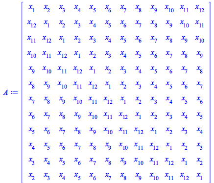
The last example is the determinant of a generic circulant matrix, i.e., where all entries are indeterminates, and each row is a cyclic rotation of the first one.
> |
 |
> |
![A := Matrix(12, shape = Circulant[[seq(x[j], j = 1 .. 12)]])](Performance/Performance_42.gif) |
> |
 |
> |
 |
This factorization took about 17 seconds in Maple 2018.
> |
 |
memory used=488.25MiB, alloc change=-41.44MiB, cpu time=5.37s, real time=3.96s, gc time=421.20ms |
> |
 |
> |
![map(nops, [op(F)])](Performance/Performance_50.gif) |
> |
![map(degree, [op(F)])](Performance/Performance_52.gif) |
> |
 |
Graph Theory
In Maple 2019 the MaximumClique function of the GraphTheory package has new algorithms for computing the maximum clique of a graph and an option to choose the algorithm that you want to use, giving a huge performance boost on certain kinds of graphs. In the following example, Maple 2019 almost instantly finds the maximum clique of a graph that Maple 2018 needed over 3 minutes to find. In this case the "sat" method is used which translates the problem into Boolean logic and solves the resulting satisfiability problem using a SAT solver.
> |
 |
> |
 |
> |
 |
> |
 |
> |
 |
memory used=10.44MiB, alloc change=28.99MiB, cpu time=187.00ms, real time=152.00ms, gc time=62.40ms |
![Typesetting:-mprintslash([C := [2, 3, 4, 6, 10, 14, 17, 20, 24, 25, 30, 33, 36, 39, 41, 45]], [[2, 3, 4, 6, 10, 14, 17, 20, 24, 25, 30, 33, 36, 39, 41, 45]])](Performance/Performance_65.gif) |
> |
 |
Group Theory
- Arithmetic and other low-level operations for permutations have been completely re-written in compiled kernel code. In addition, the memory overhead of permutations has been considerably reduced.
- For example, the following call to PermOrder took about 200 times longer in Maple 2018.
> |
 |
> |
 |
> |
 |
- Timing details will of course vary from one machine to another, and depend also upon the random state of the Maple session. But, reproduced here are some representative calculations run in a fresh Maple 2018 session, on a particular 64-bit Linux workstation.
> |
![L := CodeTools:-Usage(([seq])(Perm(combinat:-randperm(`^`(10, 4))), i = 1 .. 1000)); -1](Performance/Performance_72.gif) |
> |
 |
> |
 |
> |
 |
> |
 |
> |
 |
- And here are the same calculations run in a fresh 2019 session on the same machine. It is apparent that both time used an memory consumption have been considerably reduced.
> |
![L := CodeTools:-Usage(([seq])(Perm(combinat:-randperm(`^`(10, 4))), i = 1 .. 1000)); -1](Performance/Performance_83.gif) |
> |
 |
> |
 |
> |
 |
> |
 |
> |
 |
Real Root Finding
The RootFinding:-Isolate command has a new algorithm for univariate polynomials that is much faster for ill-conditioned problems and high accuracy solutions.